Overview
Give a high-level overview of what you implemented in this project. Think about what you've built as a whole.
Share your thoughts on what interesting things you've learned from completing the project.
In Part 1, our primary objective was to establish a mass-and-string system model. We achieved this by creating a
uniformly distributed mass grid and introducing structural, shearing, and bending constraints. These constraints
were efficiently incorporated using the "emplace_back()" function.
In Part 2, our focus shifted to cloth simulation through integration, taking into account the forces of gravity and
spring constraints. We calculated the force for each mass point using loop traversal and Hooke's Law. The positions
were then updated employing the Verlet integration formula, and spring constraints were maintained by adjusting the
particle positions as needed.
Part 3 dealt with handling collisions between the cloth and external objects like spheres or planes. For sphere
collisions, we determined the contact by comparing the distance from the mass point to the sphere's center and
adjusted the position based on frictional forces. Plane collisions were handled by projecting the mass points'
positions and correcting them if necessary, based on their orientation relative to the plane.
In Part 4, we tackled the simulation of cloth self-collisions. This involved initially calling the hash_position()
function to obtain a unique identifier for 3D coordinates. We then built a spatial map for all point masses using
the build_spatial_map() function. The self-collide function was employed to check if point masses were within a 2 *
thickness distance of each other. If so, we computed and applied an average correction for each candidate point mass
to the concerned point mass.
Part 5 saw the implementation of various shading techniques: Diffuse Shading, Blinn-Phong Shading, Texture Mapping,
Bump Mapping, Displacement Mapping, and Environment Mapped Reflections. Diffuse shading was achieved using the
standard formula for diffuse lighting. Blinn-Phong Shading incorporated ambient, diffuse, and specular components.
Texture Mapping involved sampling from a texture at coordinates (u, v). Bump Mapping entailed modifying normal
vectors to create the illusion of surface texture. Displacement Mapping altered vertex positions according to a
height map, changing the object's geometry and adjusting normals accordingly. Environment Mapped Reflections used
pre-computed direction-to-radiance mappings from an environment map, sampling it based on the direction of the
incoming light wi relative to the outgoing eye-ray wo.
Part 1: Masses and springs
Take some screenshots of scene/pinned2.json from a viewing angle where you can clearly see the cloth wireframe to
show the structure of your point masses and springs.
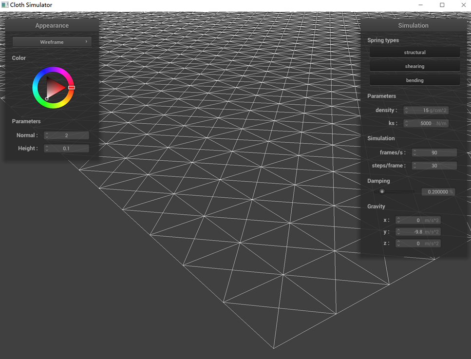
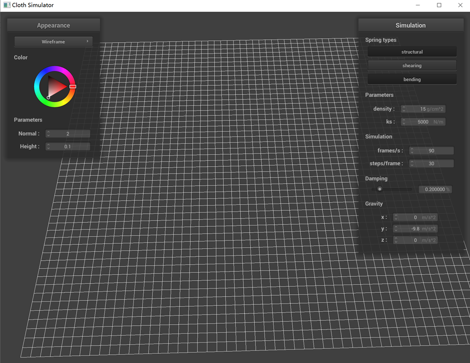
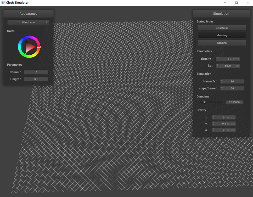
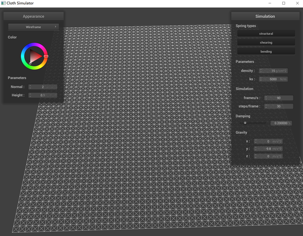
Show us what the wireframe looks like (1) without any shearing constraints, (2) with only shearing constraints,
and (3) with all constraints.
 (1) without any shearing constraints
|
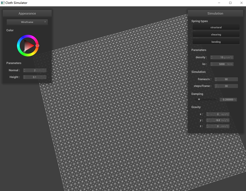
 (2) with only shearing constraints
|
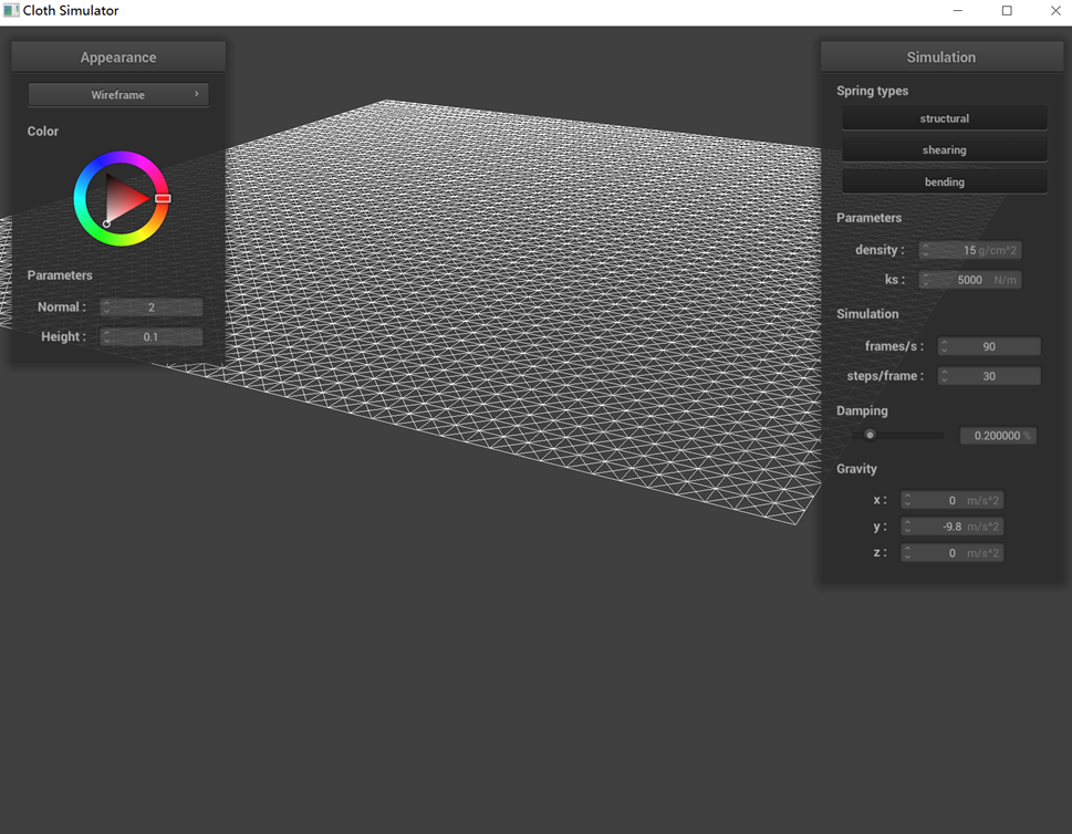
 (3) with all constraints
|
In the scenario where all constraints are applied, each cell within the mesh is characterized by having not only
four sides but also diagonal elements. However, upon removing the shearing constraints, the mesh's diagonal
elements vanish. This change occurs because, in our model, shearing constraints are implemented by applying them
between a point and its top-left and top-right neighbors, resulting in diagonal connections. In the absence of
these constraints, the mesh loses its ability to resist shearing forces.
Similarly, when the structural constraints are removed, the four sides of each mesh cell disappear, leaving only
the diagonal elements intact. This happens because the structural constraints in our design are applied between a
point and its immediate left and top neighbors, creating the mesh's four-sided structure.
Part 2: Simulation via numerical integration
Experiment with some the parameters in the simulation. To do so, pause the simulation at the start with P, modify
the values of interest, and then resume by pressing P again. You can also restart the simulation at any time from
the cloth's starting position by pressing R.
Describe the effects of changing the spring constant ks; how does the cloth behave from start to rest
with a very low ks? A high ks?
What about for density?
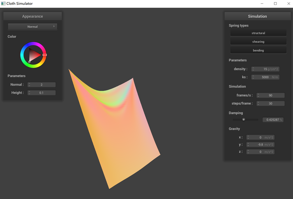
What about for damping?
For each of the above, observe any noticeable differences in the cloth compared to the default parameters and
show us some screenshots of those interesting differences and describe when they occur.
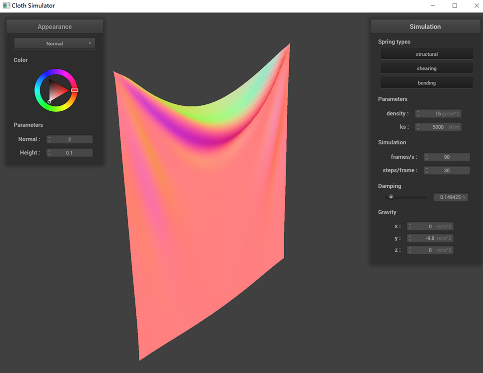
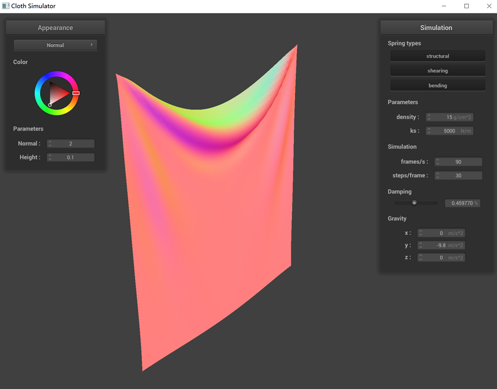
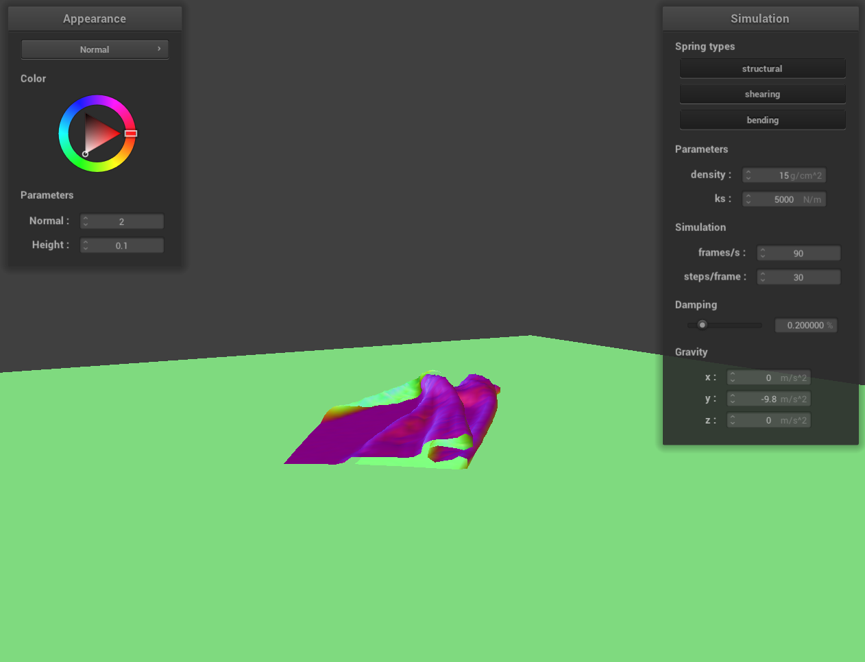
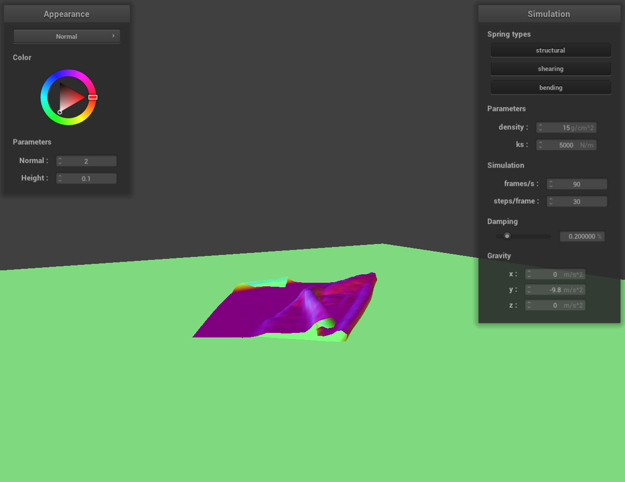
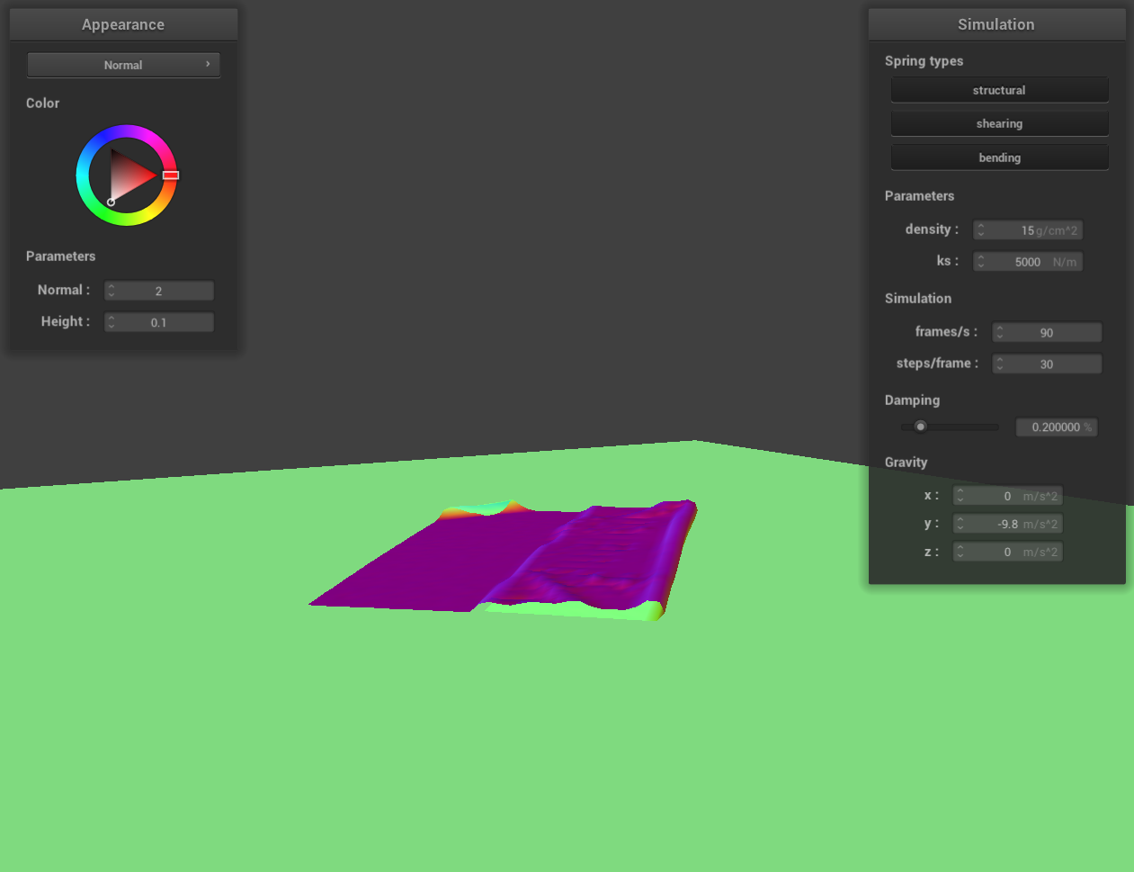
The performance of a pinned cloth simulation under various parameters (ks, density, damping) is demonstrated
below, with the default settings being ks=5000, density=15, and damping=0.2%.
(1) Observations from the graph when adjusting only ks reveal that at lower ks values, the cloth exhibits more
pronounced wrinkles, whereas at higher ks values, it appears relatively flat. This variation is due to the
decrease in stiffness with lower ks, rendering the cloth softer and more prone to bending. Conversely, a higher ks
value results in a stiffer cloth that resists bending.
(2) Modifying only the density parameter, the graph shows that a higher density results in the cloth hanging
more prominently, whereas at lower densities, this effect is less noticeable. This is because an increase in
density leads to a heavier cloth, which is more influenced by gravity and thus more likely to deform.
(3) Changes in damping, as reflected in the graph, do not alter the final state of the cloth. However,
reducing the damping value lessens the resistance to cloth movement, making it more susceptible to swaying and
taking longer to cease motion. Screenshots illustrating the cloth's behavior under different damping values show
that lower damping results in more unstable and significantly swaying cloth motions.
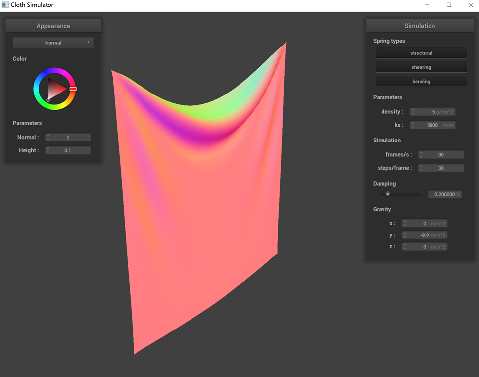 ks = 5000 N/m (default)
|
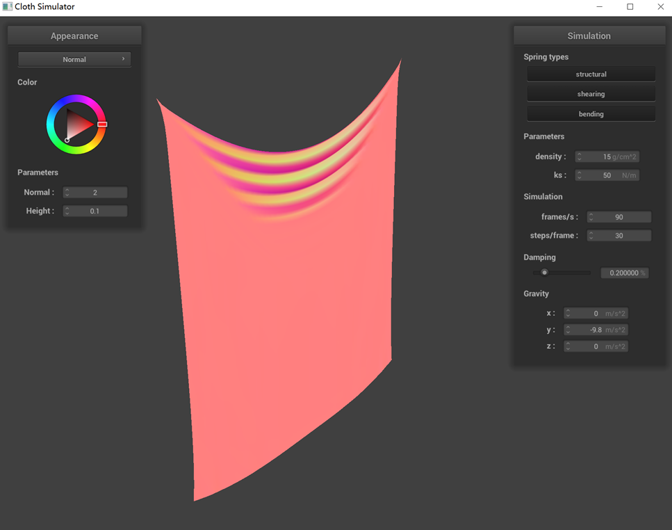 ks = 50 N/m
|
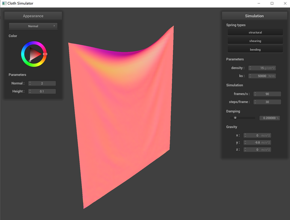 ks = 50000 N/m
|
 density = 15 g/cm^3 (default)
|
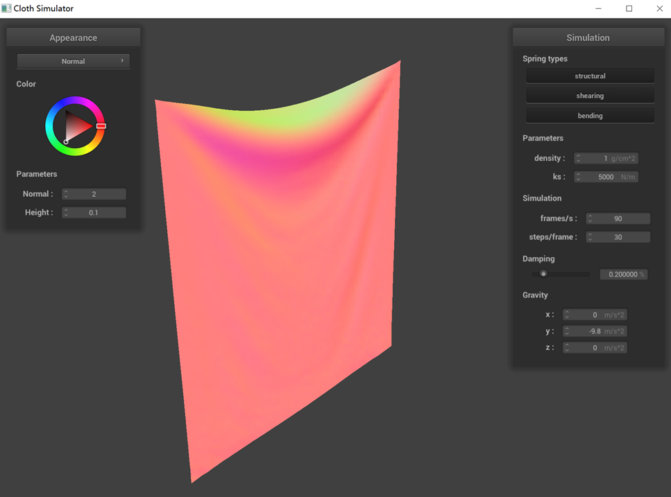 density = 1 g/cm^3
|
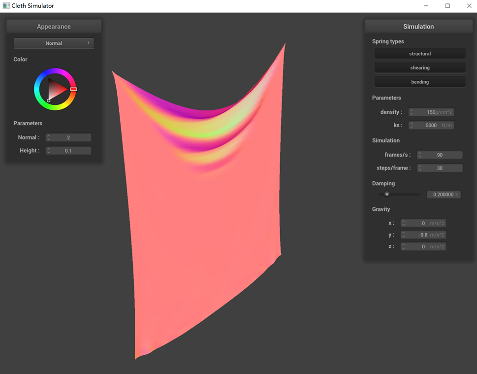 density = 150 g/cm^3
|
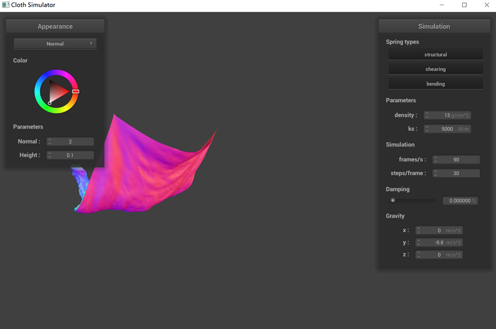 small damping (Intermediate state)
|
 large damping (Intermediate state)
|
 small damping (Final state)
|
 large damping (Final state)
|
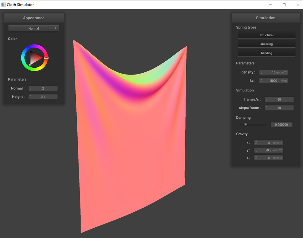
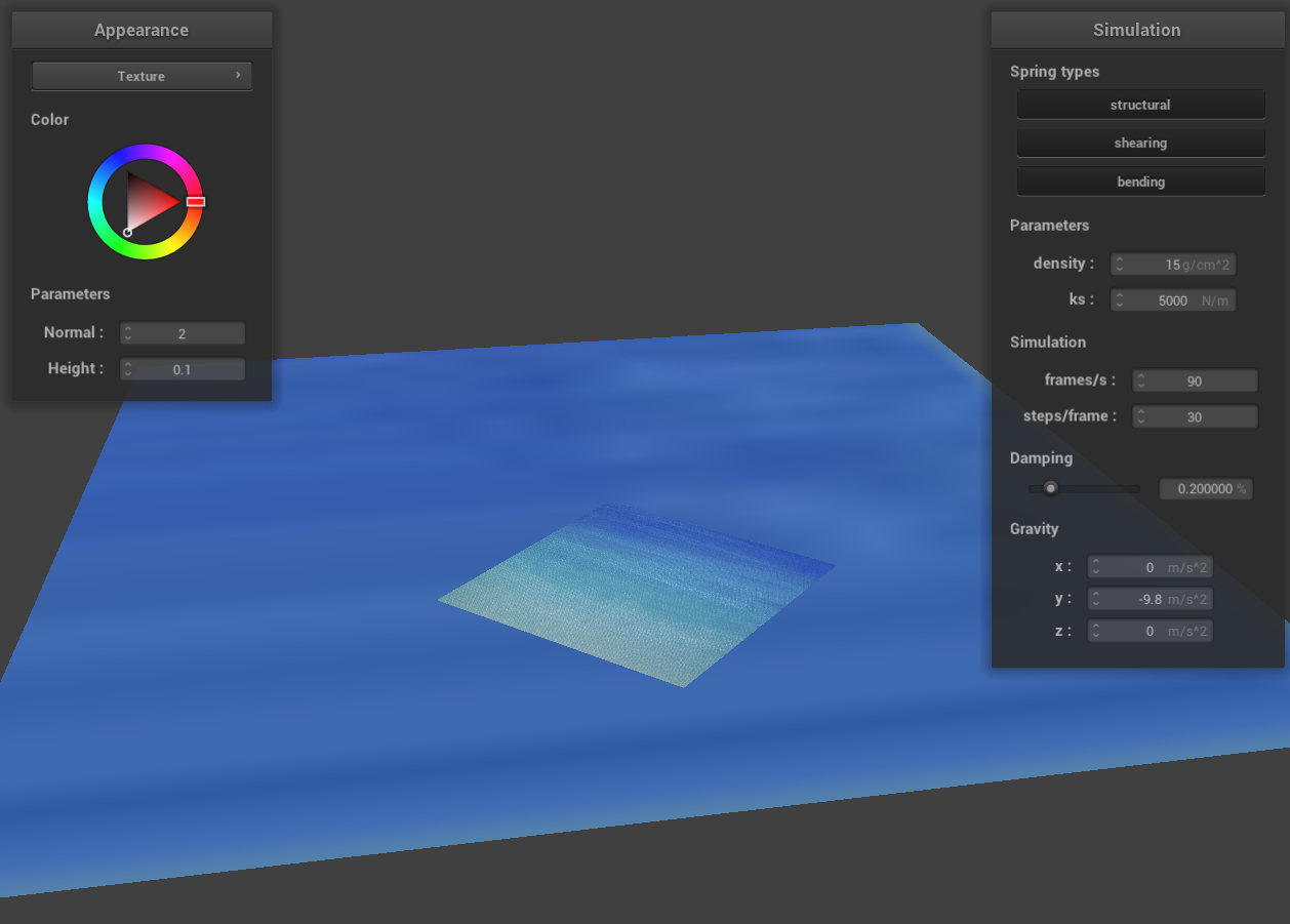
Show us a screenshot of your shaded cloth from scene/pinned4.json in its final resting state! If you choose to
use different parameters than the default ones, please list them.
The image of the shaded cloth in pinned4.json is shown below. All the parameters are the default ones.
Part 3: Handling collisions with other objects
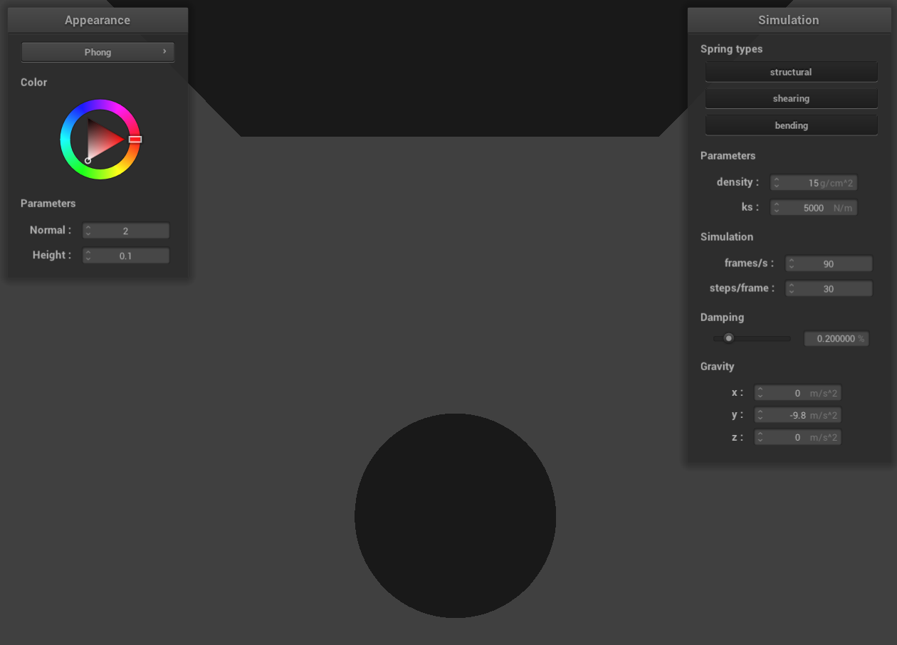
Show us screenshots of your shaded cloth from scene/sphere.json in its final resting state on the sphere using
the default ks = 5000 as well as with ks = 500 and ks = 50000. Describe the differences in the results.
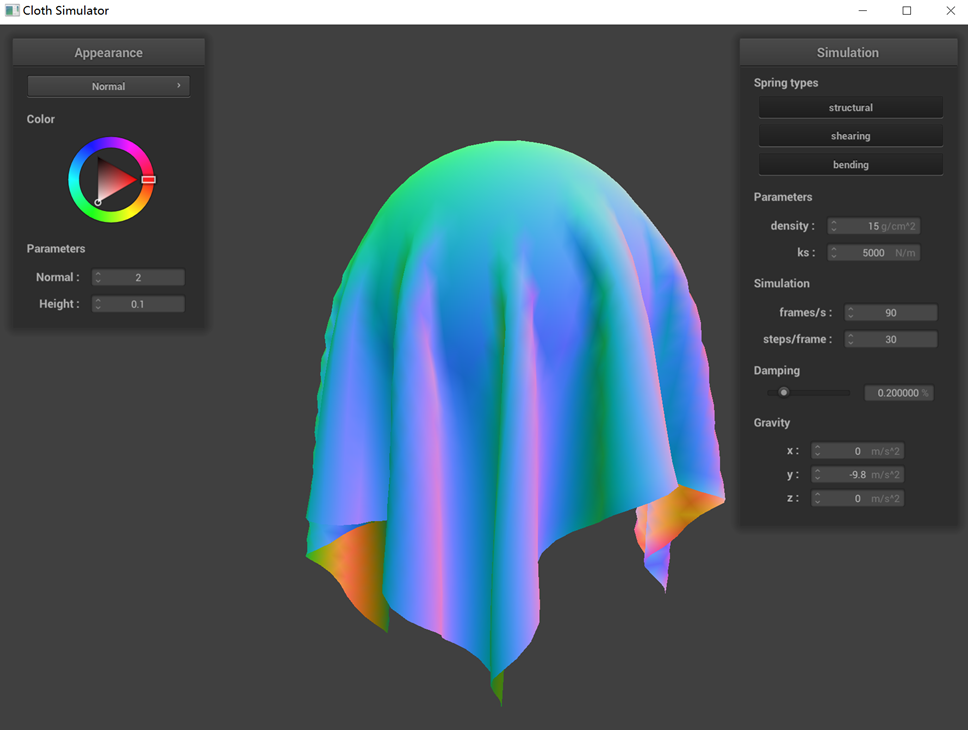 ks = 5000 N/m
|
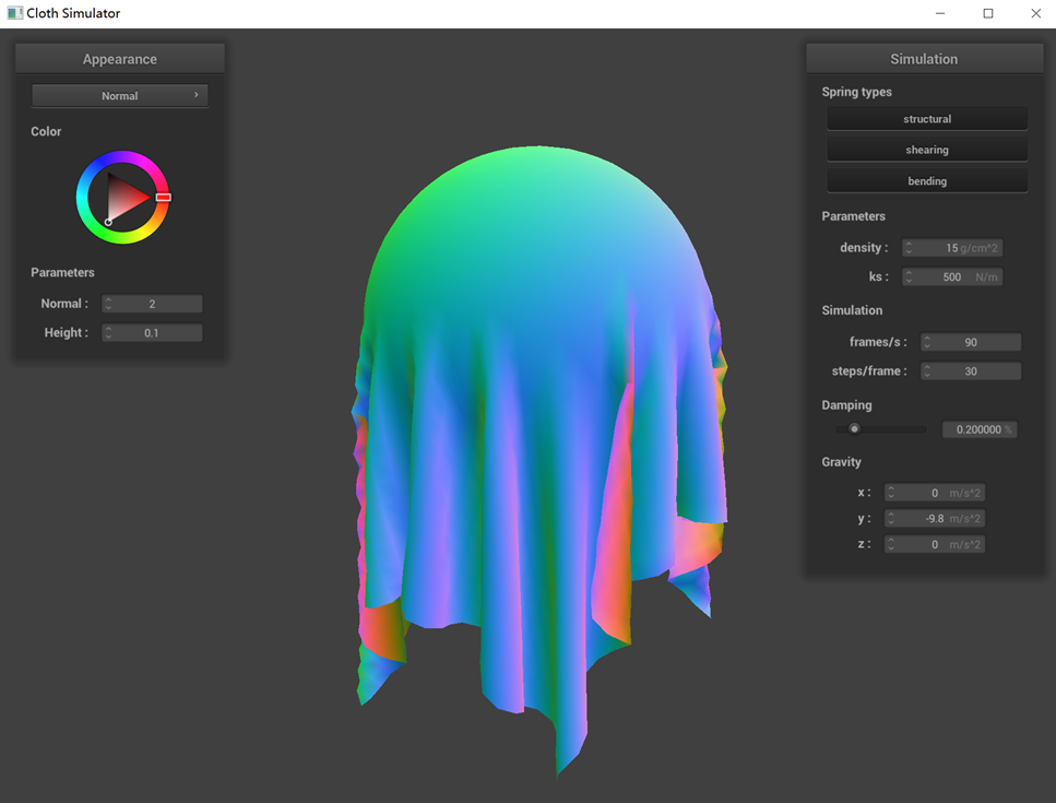 ks = 500 N/m
|
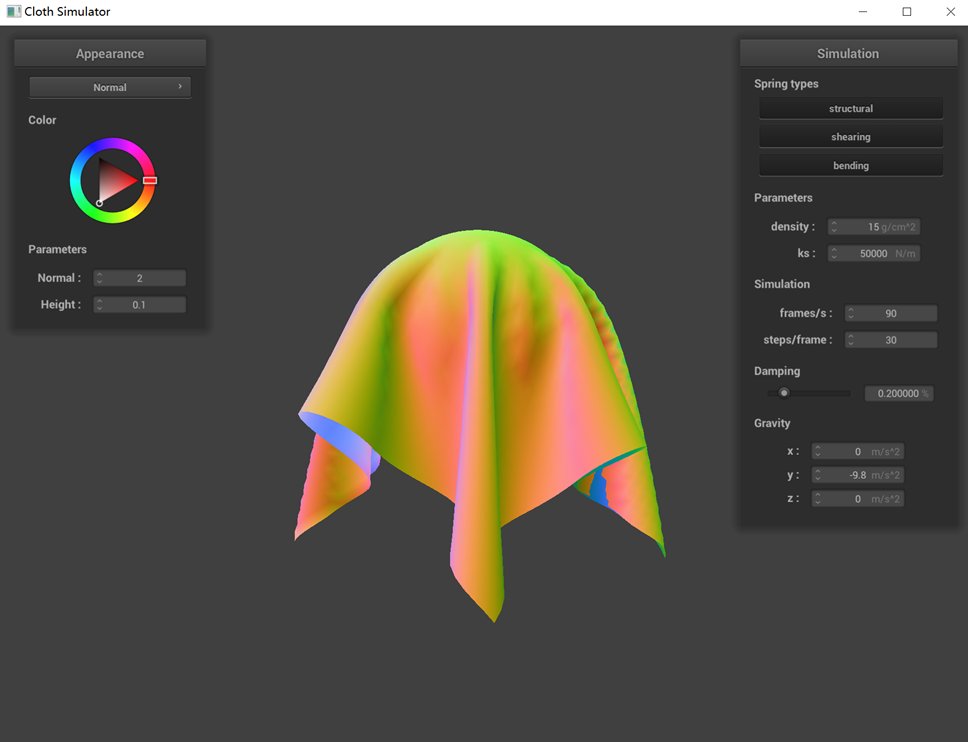 ks = 50000 N/m
|
The collision dynamics between the cloth and the sphere are noticeably influenced by different ks values. With a
lower ks value, such as 500, the cloth exhibits reduced surface elasticity, leading to a less pronounced ability
to bounce back. This results in a softer appearance, with the cloth more readily adhering to the sphere upon
contact. Conversely, at a higher ks value like 50000, the cloth experiences a stronger rebound force during
collisions. This increased force causes the cloth to be more forcefully repelled away from the sphere.
Show us a screenshot of your shaded cloth lying peacefully at rest on the plane. If you haven't by now, feel
free to express your colorful creativity with the cloth! (You will need to complete the shaders portion first to
show custom colors.)
Part 4: Handling self-collisions
Show us at least 3 screenshots that document how your cloth falls and folds on itself, starting with an early,
initial self-collision and ending with the cloth at a more restful state (even if it is still slightly bouncy on
the ground).
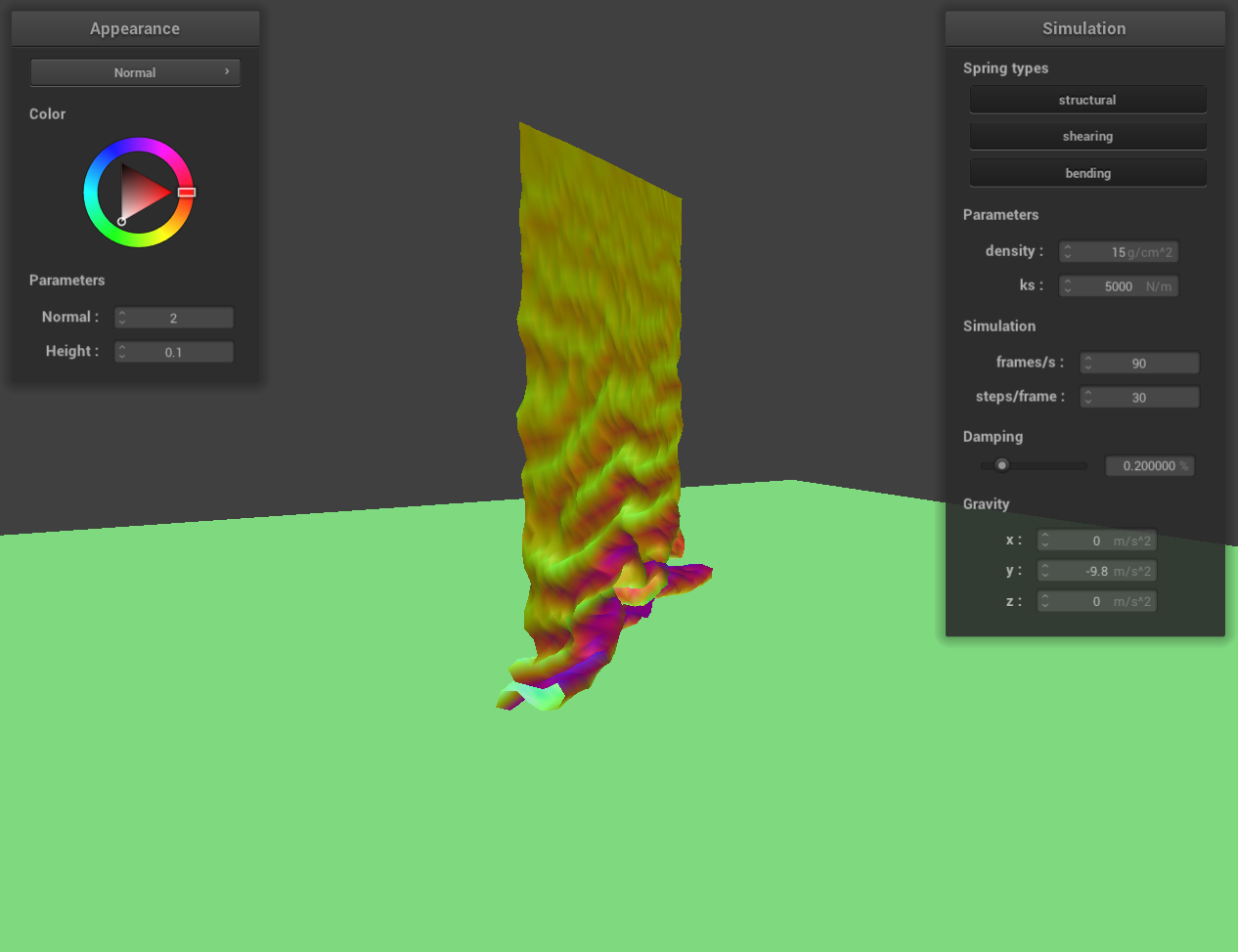 screenshot 1
|
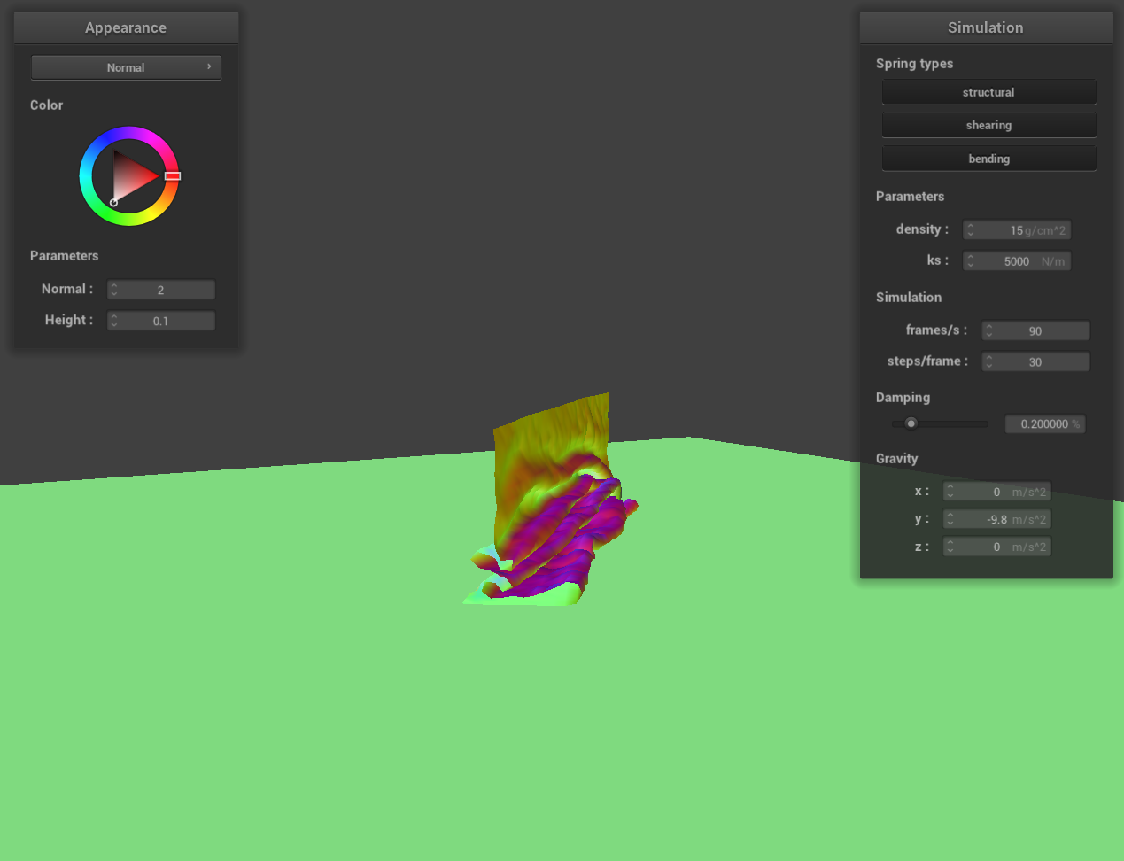 screenshot 2
|
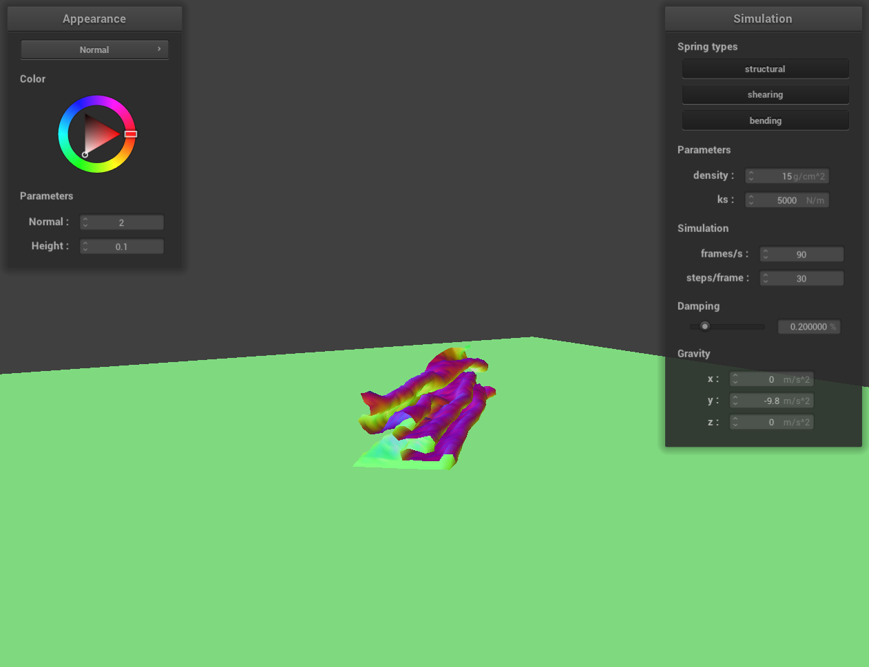 screenshot 3
|
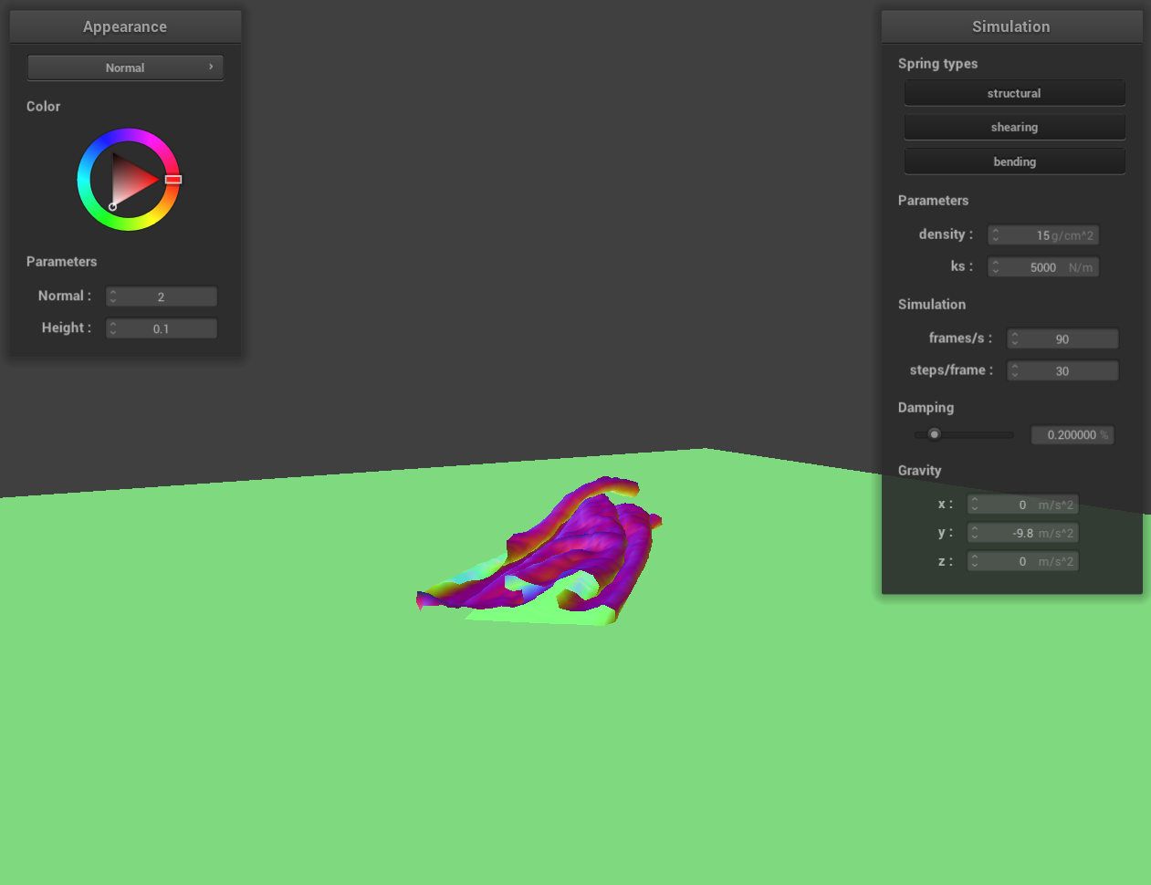 screenshot 4
|
 screenshot 5
|
 screenshot 6
|
 screenshot 7
|
 screenshot 8
|
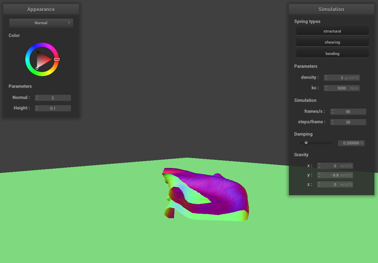
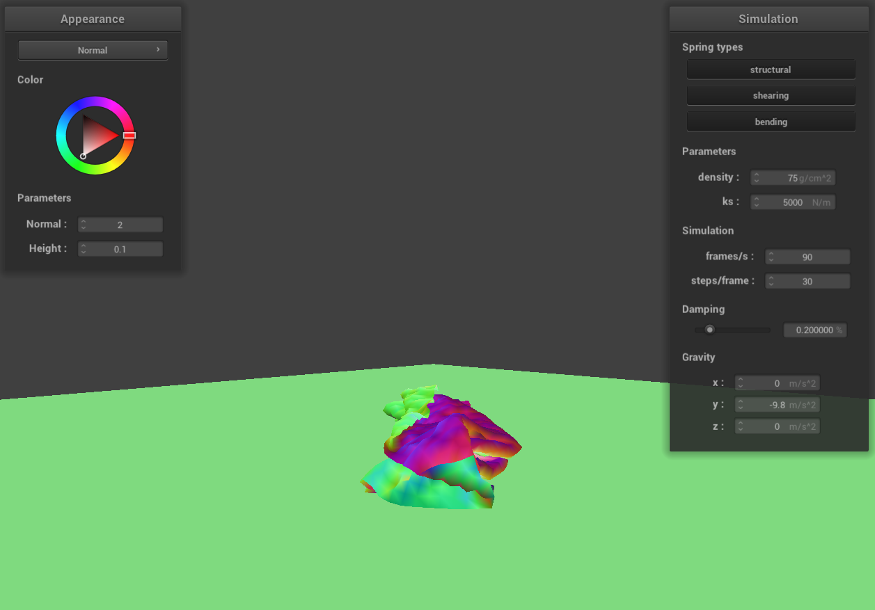
Vary the density as well as ks and describe with words and screenshots how they affect the behavior of the cloth
as it falls on itself.
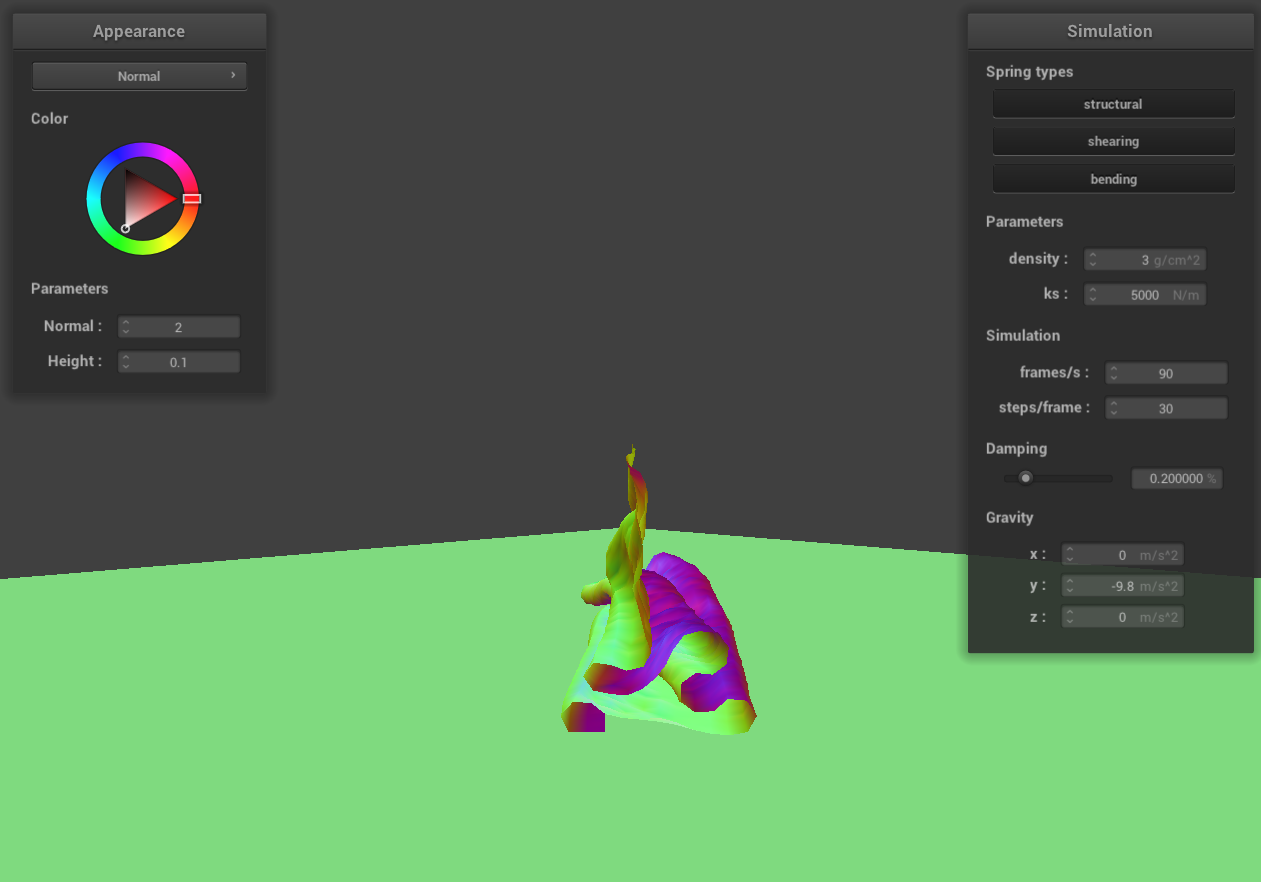 density = 3 g/cm^3
|
 density = 3 g/cm^3
|
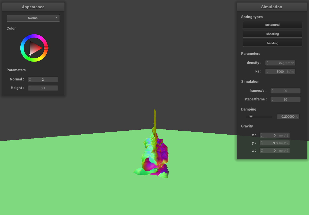 density = 75 g/cm^3
|
 density = 75 g/cm^3
|
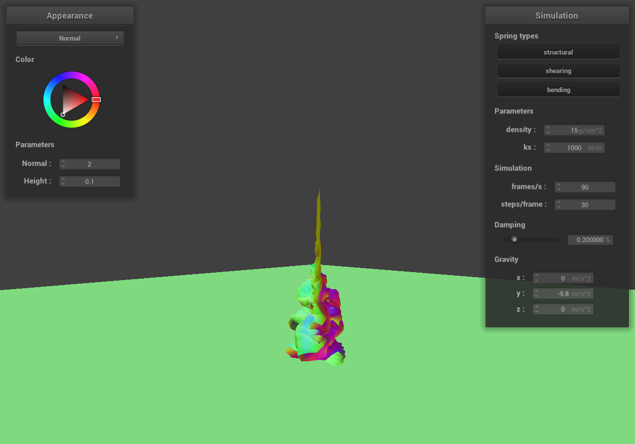 ks = 1000 N/m
|
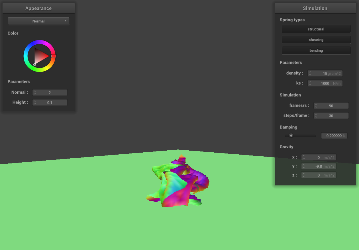 ks = 1000 N/m
|
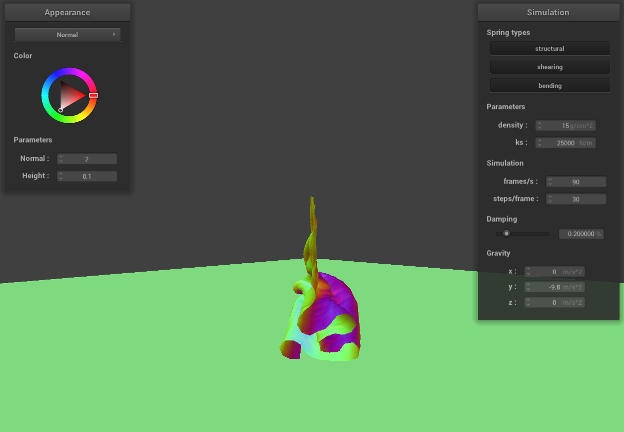 ks = 25000 N/m
|
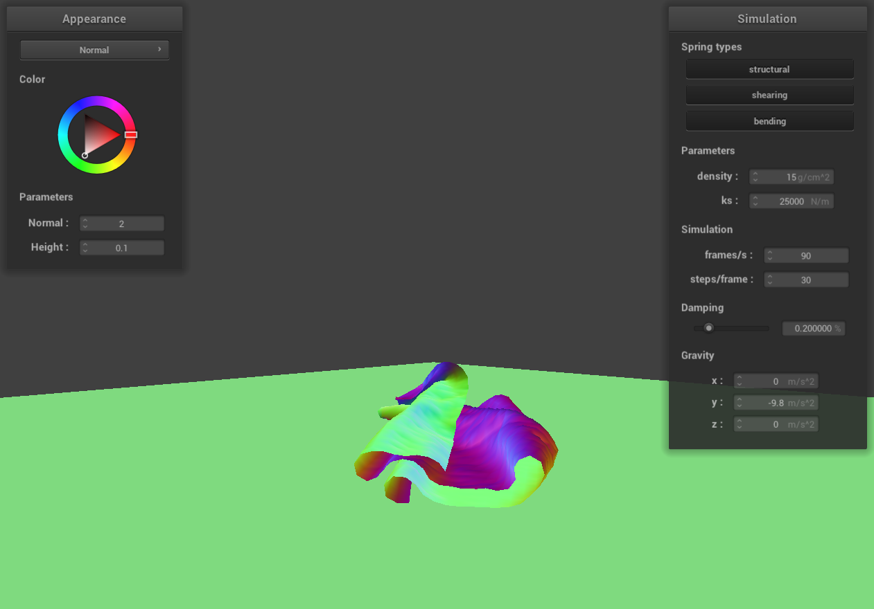 ks = 25000 N/m
|
When we decrease the density while keeping ks constant, the cloth tends to fall more loosely upon itself. This is
due to the reduced gravitational pull on the cloth, while the elastic force exerted by its fibers remains
unchanged. In contrast, increasing the density, with ks unchanged, results in the cloth becoming more compact as
it falls. This compactness is a consequence of the increased gravitational force acting on the cloth, while the
elastic force is still constant.
Similarly, decreasing ks while maintaining the same density leads to a more compact fall of the cloth. This
effect arises because the decrease in ks reduces the elastic force within the cloth, while the gravitational pull
remains constant. On the other hand, increasing ks, with density remaining the same, causes the cloth to fall more
loosely. This looser fall is due to the increased elastic force counteracting the unchanged gravitational
influence.
Part 5: Shaders
Explain in your own words what is a shader program and how vertex and fragment shaders work together to create
lighting and material effects.
Shader programs are integral to the graphics rendering pipeline, where they are employed to process vertices and
pixels. Running parallel in the GPU, these programs are pivotal in computer graphics and game development, tasked
with managing lighting, textures, and colors on the surfaces of 3D models to produce the final visual effects.
Typically, shader programs comprise two main components: the vertex shader and the fragment shader.
Vertex shaders handle the processing of each vertex in a 3D model. Their responsibilities include applying
transformations to vertices, calculating their screen positions, and executing calculations for attributes like
lighting and normals. The vertex shader outputs the final position of each vertex to gl_Position and generates
varying values for use in the fragment shader. The results from these calculations are then forwarded to the
fragment shader.
Fragment shaders, on the other hand, are tasked with determining the color and texture information for each pixel.
After rasterization, fragments are processed by these shaders. Utilizing the data received from the vertex shader,
typically encompassing geometric attributes, fragment shaders compute the final color value for each pixel. This
computation culminates in the rendering of the final image, with the color being written into out_color.
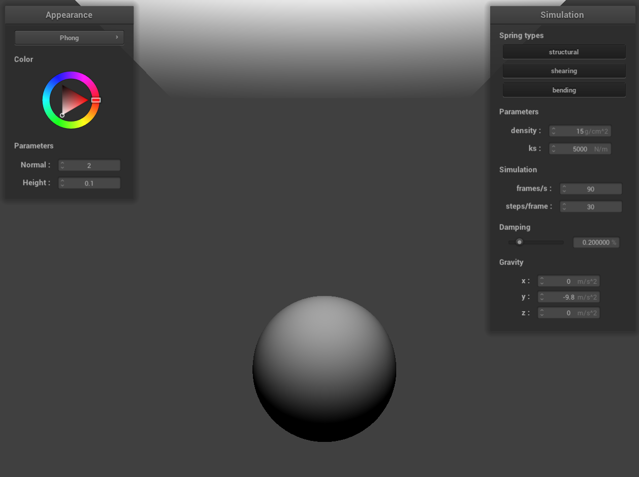
Explain the Blinn-Phong shading model in your own words. Show a screenshot of your Blinn-Phong shader outputting
only the ambient component, a screen shot only outputting the diffuse component, a screen shot only outputting the
specular component, and one using the entire Blinn-Phong model.
The Blinn-Phong shading model is a classical and widely adopted illumination model in computer graphics. It
calculates the color at each point on an object's surface using three components: ambient, diffuse, and specular.
The Blinn-Phong shading model's equation is L = ka * Ia + kd * (I / r^2) * max(0, n * l) + ks * (I / r^2) * max(0,
n * h)^p, which aggregates the contributions from the ambient, diffuse, and specular components.
The ambient component accounts for the illumination of the object’s surface in the absence of direct light
sources. Typically a constant value, it simulates the effects of indirect lighting that illuminates the object
evenly, regardless of its orientation or location.
The diffuse component reflects the illumination on the object’s surface under direct light. It is influenced by
the direction of the surface normal, the direction of the light source, and the object's color and texture.
Diffuse illumination is uniformly distributed across the surface and remains constant, irrespective of the
viewer’s perspective.
Lastly, the specular component is responsible for the glossy reflections observed on the smooth parts of an
object’s surface. It depends on the direction of the surface normal, the light source, the viewer's angle, and the
object's specular reflection coefficient. The Blinn-Phong model employs a halfway vector to streamline the
calculation of specular reflection, enhancing computational efficiency.
 only the ambient component
|
 only the diffuse component
|
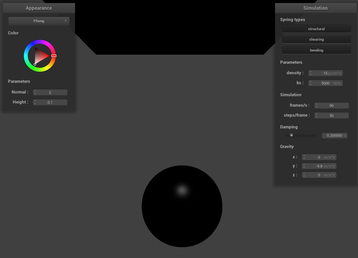 only the specular component
|
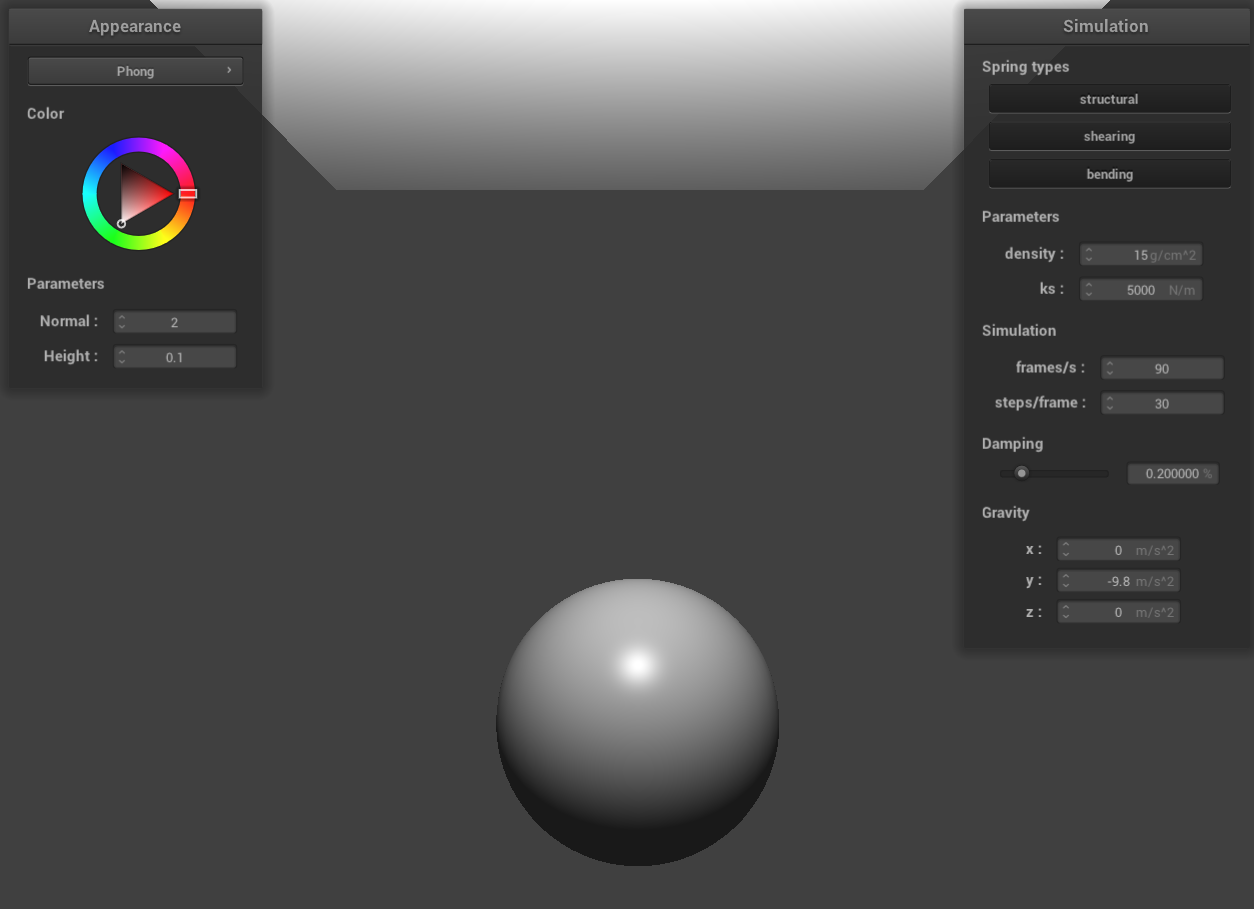 the entire Blinn-Phong model
|
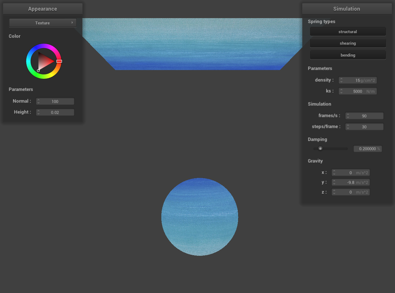
Show a screenshot of your texture mapping shader using your own custom texture by modifying the textures in
/textures/.
Show a screenshot of bump mapping on the cloth and on the sphere. Show a screenshot of displacement mapping on
the sphere. Use the same texture for both renders. You can either provide your own texture or use one of the ones
in the textures directory, BUT choose one that's not the default texture_2.png. Compare the two approaches and
resulting renders in your own words. Compare how your the two shaders react to the sphere by changing the sphere
mesh's coarseness by using -o 16 -a 16 and then -o 128 -a 128.
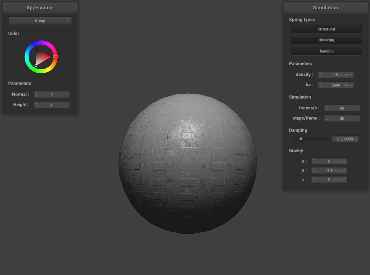
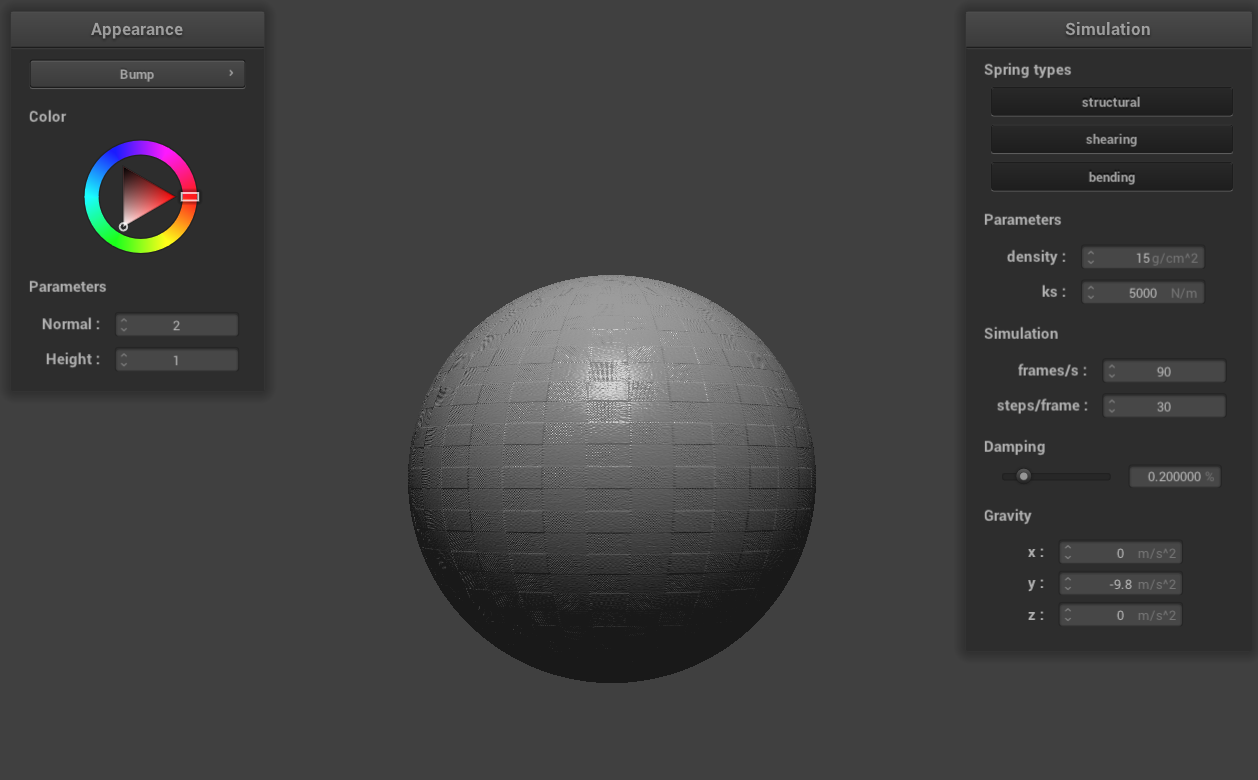
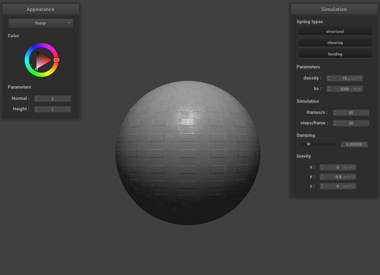 bump mapping on the sphere
|
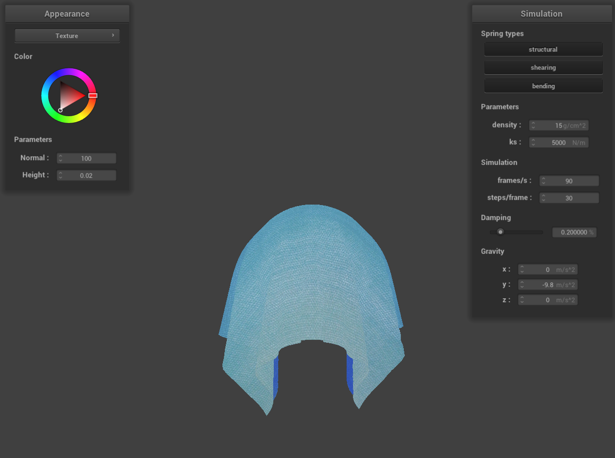
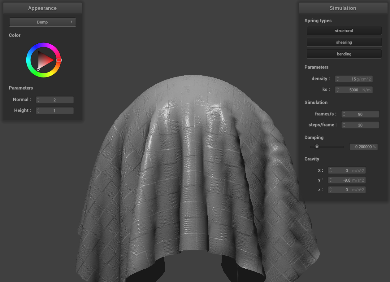 bump mapping on the cloth
|
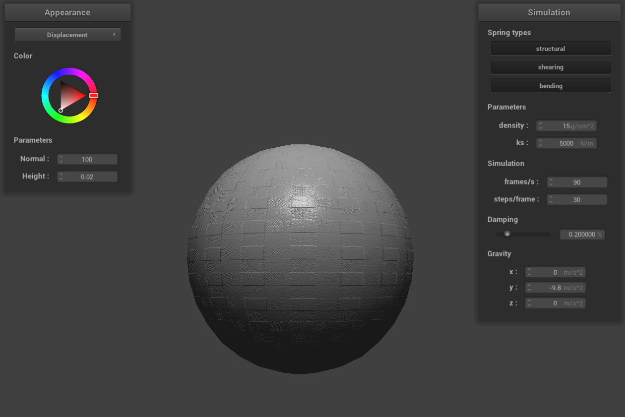
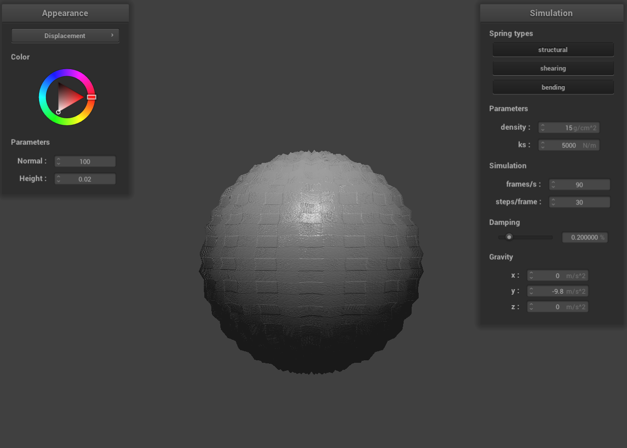 displacement mapping on the sphere
|
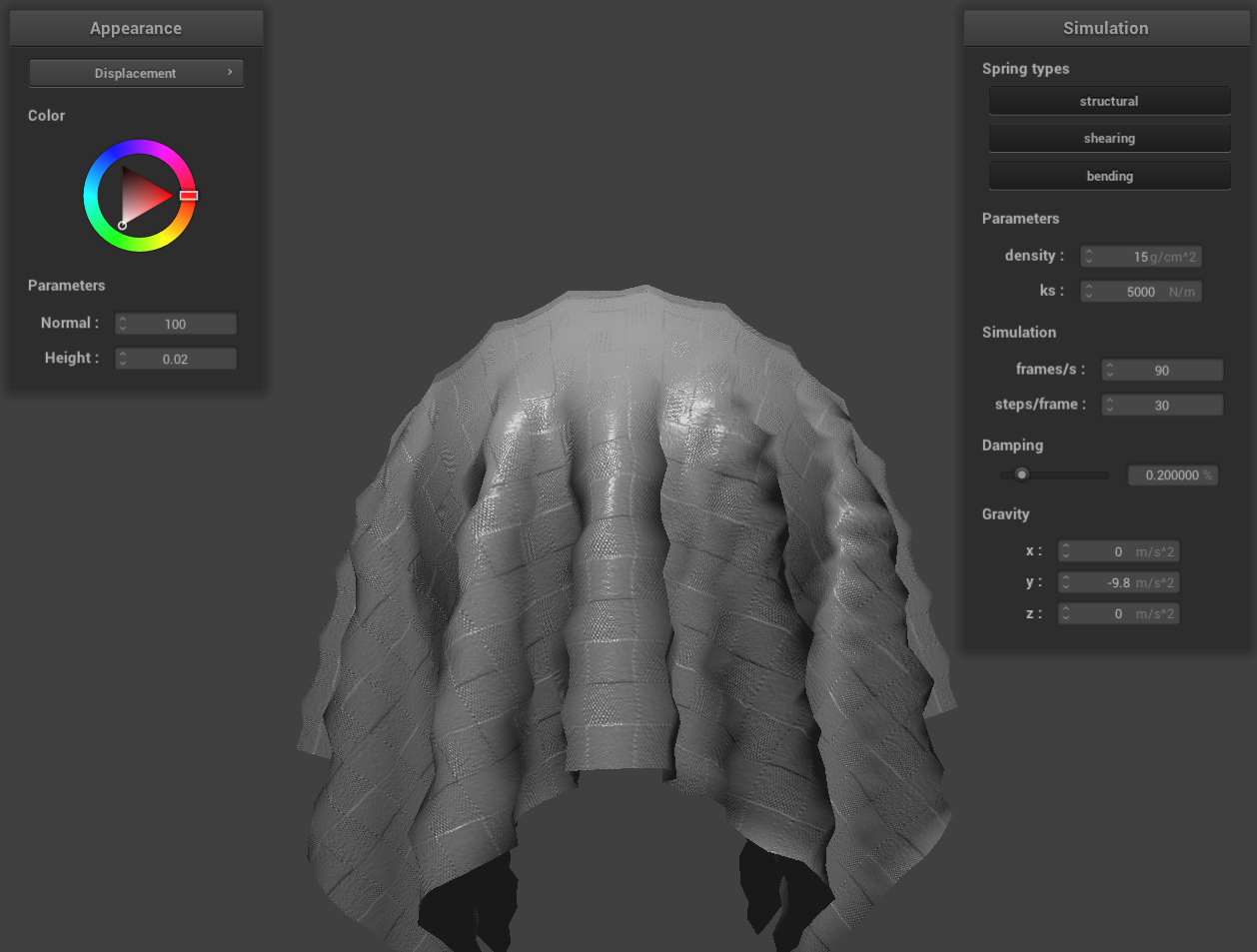 displacement mapping on the cloth
|
Bump mapping is a technique used to simulate the appearance of bumps and irregularities on an object's surface. It
achieves this by altering the normal vectors of the object. The fragment shader then creates an illusion of
textured bumps, enhancing the visual complexity of the surface. Importantly, bump mapping only affects the surface
lighting during rendering and does not modify the actual geometry of the object.
Displacement mapping, on the other hand, is a more sophisticated technique that adds surface detail by physically
altering the object's geometry. It achieves this by adjusting the vertices' positions to reflect a height map,
along with corresponding modifications to the normals to align with the new geometry. During rendering, the
displacement map reshapes the object's vertices based on height values. This alteration of the actual geometry
allows for the creation of realistic details that are visible from any viewing angle.
In renders utilizing bump mapping, the geometry of the sphere and the cloth remains unchanged. The technique
modifies the surface lighting to create the illusion of bumps on these objects.
In contrast, renders employing displacement mapping show noticeable changes in the geometry of the sphere and the
cloth. This geometric alteration affects the surface normals, which in turn influences the objects' interaction
with lighting. The change in surface normals leads to corresponding adjustments in surface lighting, enhancing the
realism of the rendered objects.
 bump mapping -o 16 -a 16
|
 bump mapping -o 128 -a 128
|
 displacement mapping -o 16 -a 16
|
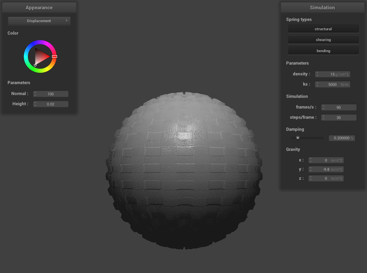 displacement mapping -o 128 -a 128
|
In the case of bump mapping, altering the coarseness of the sphere mesh using parameters -o 16 -a 16 and then -o
128 -a 128 does not lead to significant changes in the rendered sphere. This outcome is attributed to bump
mapping's approach of simulating bumps and irregularities by modifying surface normals instead of altering the
object's actual geometry. As a result, increasing the mesh resolution does not have a substantial impact on the
calculation of surface normals in bump mapping.
However, with displacement mapping, the rendered sphere undergoes considerable changes when varying the mesh's
coarseness with the same parameters. Notable alterations in the sphere's geometry are evident. This is because
displacement mapping enhances surface detail by physically modifying the object's geometry, which often requires
more vertex data for accurately capturing surface details. At lower resolutions, the effectiveness of displacement
mapping can be limited as it struggles to adequately represent the height variations on the object's surface.
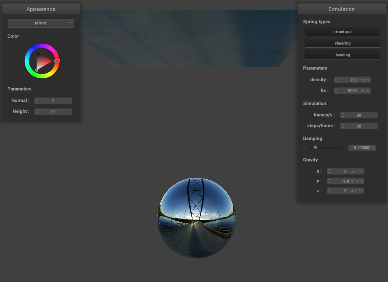
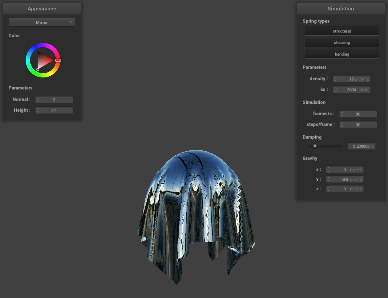
Show a screenshot of your mirror shader on the cloth and on the sphere.