For this assignment I implemented a forward-rendering lighting system on top of the existing Vulkan pipeline.
Light data (sphere, spot, and sun lights) is loaded from the LIGHT entries in the s72 scene file into a flat Light struct array (position/type, direction/shadow-slot, tint×power, and per-type parameters) and uploaded every frame as a storage buffer.
The fragment shader loops over all lights and accumulates contributions using a Lambertian diffuse term and a GGX/Smith PBR BRDF, with environment-map IBL as a base.
For shadows, a dedicated ShadowPipeline renders depth to a R32_SFLOAT color attachment for up to 8 spot lights per frame; the shadow maps are then sampled with 4-sample PCF and a constant depth bias.
The extra-credit features A3x-sort, A3x-soft, A3x-cascade, and A3x-cube were not completed due to time constraints.
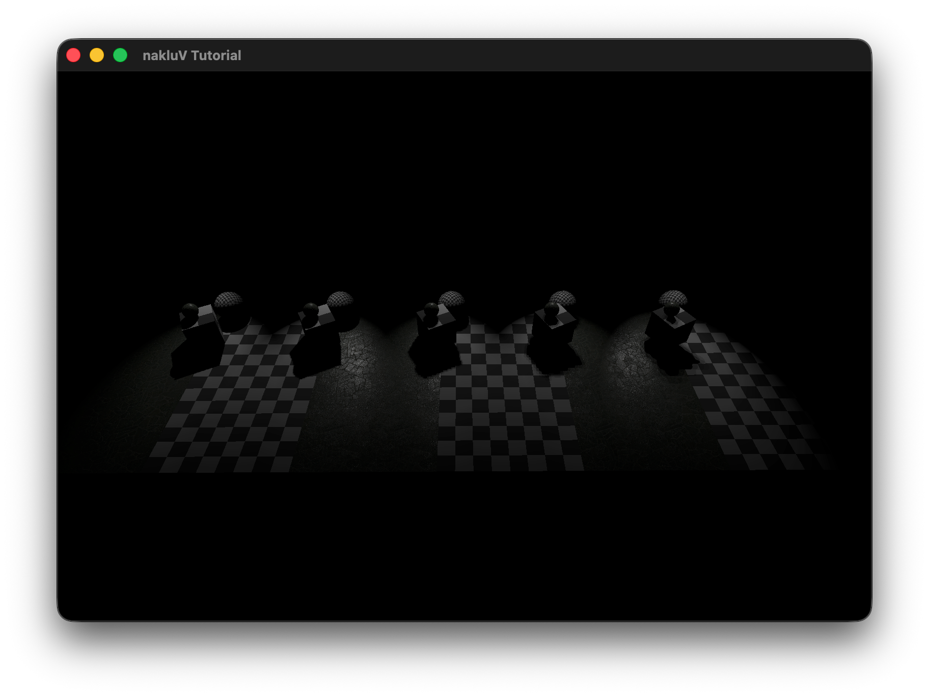
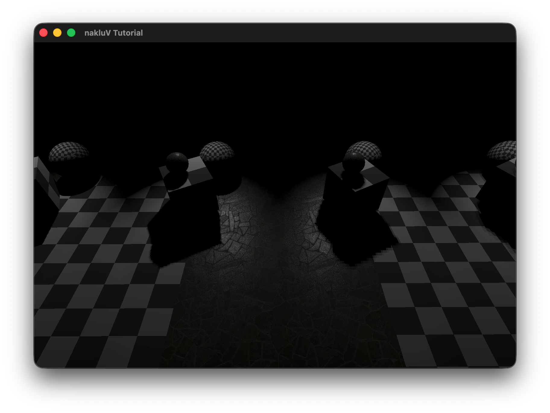
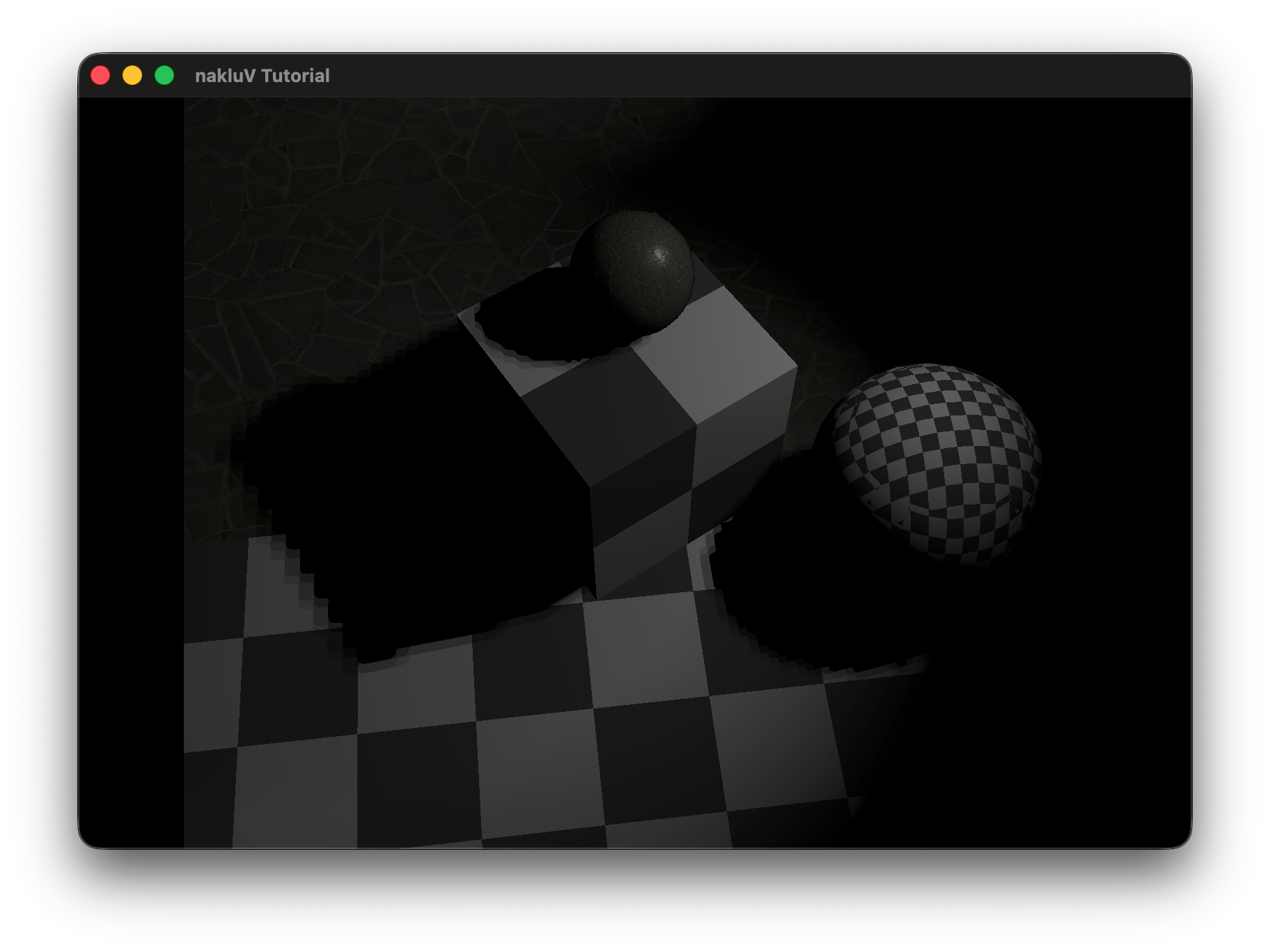
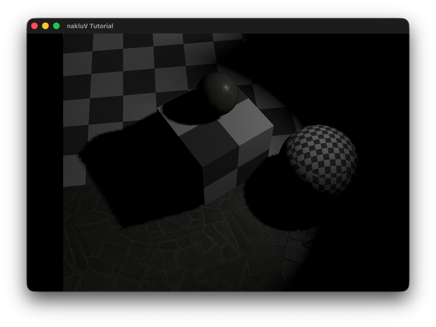
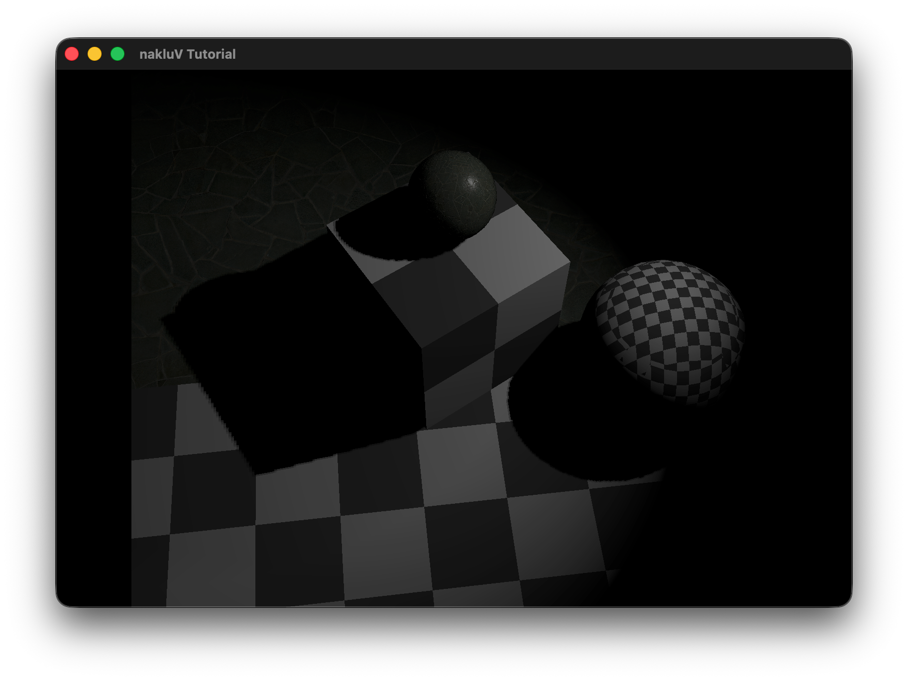
Describe the scene you lit, the light count and placement approach, and include a screen recording showing it running in real-time:
Credit + cite your sources for textures and models, if you did not create them yourself.
Document the command-line arguments that can be used to control your viewer. This will probably be a copy of the section from your A2 report with a few new flags relating to lights (if you added any).
--scene scene.s72 -- required -- load scene from scene.s72--camera name -- optional -- view the scene through the camera name--physical-device name -- optional -- use the physical device whose VkPhysicalDeviceProperties::deviceName matches name--drawing-size w h -- optional -- set the initial size of the drawable part of the window in physical pixels of width w and height h--culling mode -- optional -- sets the culling mode to be none|frustum|bvh--headless -- optional -- if specified, run in headless mode (no windowing system connection), and read frame times and events from standard input. In headless mode, the flag --drawing-size specifies the size of the offscreen canvas that is rendered into --test mode -- optional -- runs the A1-test section, mode can be cpu or gpu
Under cpu mode, the program will automatically loads the test scene for cpu "cpu-bottleneck.s72"
Under gpu mode, the program will load the scene from --scene scene.s72 argument--culled-count number -- optional -- combined with --test cpu argument to set the number of culled objects (outside the camera frustum) in the scene--csv-file-name file_name -- optional -- in A1-test section, the user chosen log file name--exposure E
scale computed radiance by 2E before tone mapping.
This simulates camera exposure adjustment and is always applied prior to the tone-mapping operator.
--tone-map mode
select the tone-mapping operator used to convert HDR radiance to displayable color.
Supported modes are:
linear (no additional mapping after exposure) and
reinhard (nonlinear compression of high luminance values).
The purpose of this section is to get you to think critically about your code by providing evidence sufficient to demonstrate to course staff that it works. These thoughts may also help you improve the code as you work on it in the Final project and beyond.
During scene graph traversal in SceneViewer.cpp, each node that references a "LIGHT" object is parsed and stored as a LightInfo struct in a flat std::vector<LightInfo>.
The struct records the light type (sun / sphere / spot), world-space position and direction (computed from the node's transform), the tint color, and the type-specific intensity value — strength for sun lights and power for sphere and spot lights — kept as separate fields.
At render time these are repacked into GPU-side Light structs (one storage buffer per frame) where TINT_STRENGTH.xyz holds the raw tint and TINT_STRENGTH.w holds the raw power/strength; tint and power are multiplied together in the fragment shader.
The one exception is the sky/sun environment energy stored in the World uniform, where tint and strength are premultiplied into SUN_ENERGY / SKY_ENERGY at update time since those values are consumed directly without a per-light loop.
All lights are passed to materials through a single GPU-side storage buffer bound at set 0, binding 4, shared across all draw calls in a frame.
Each entry in the buffer is a 64-byte Light struct composed of four vec4s:
POSITION_TYPE (xyz = world-space position, w = type: 0=sun, 1=sphere, 2=spot),
DIRECTION_SHADOW (xyz = normalized direction, w = shadow-map slot index, or −1 if unshadowed),
TINT_STRENGTH (rgb = tint, w = power/strength),
and PARAMS (per-type parameters: cone angle, radius, range limit, blend factor).
The total light count is carried in the World uniform buffer (set 0, binding 0) as LIGHT_COUNT, so the fragment shader knows how many entries to iterate over.
Every frame, Tutorial.cpp converts the flat std::vector<LightInfo> from the scene viewer into this packed array, uploads it via a host-coherent staging buffer (Lights_src), and copies it to a device-local buffer (Lights); the descriptor is updated once when the buffer is (re)allocated and remains valid for subsequent frames until the light count grows.
The test scene consists of a single 70×70 lambertian floor plane (checker texture) with N unshadowed sphere lights (radius=0, power=200, limit=20) arranged in a uniform grid 3 units above the surface, and a fixed overhead camera at [0, 0, 50] looking straight down.
Each data point is the average gpu_draw_ms over 190 frames (first 10 warmup frames discarded), measured on Apple M3 Max via Vulkan timestamp queries.
The increase is nearly linear for N ≥ 20, as expected from the per-light loop in the fragment shader.
At the low end (N < 20) the fixed GPU overhead dominates and the curve appears flat.
Even at 1000 lights the GPU draw time is only ~4.8 ms, well under the 33 ms budget for 30 fps, so the viewer handles at least 1000 lights at a very comfortable frame rate on this hardware.
Shadow maps are rendered at the very beginning of each frame's command buffer, before the main color pass.
For each spot light whose "shadow" field is non-zero, a dedicated ShadowPipeline render pass draws all scene geometry into a shadow × shadow R32_SFLOAT color attachment (plus a D32_SFLOAT depth attachment for hardware depth testing).
Writing depth to a float color attachment — rather than sampling a depth-format image — avoids macOS/MoltenVK restrictions on depth texture sampling.
The shadow camera is set up each frame with a perspective projection whose field of view matches the spot light's fov, near plane = max(radius, 1.0), far plane = limit (or 1000 if unlimited), and a lookAt aimed along the spot's emission direction.
The world-to-clip matrix for each shadow slot is also uploaded to a ShadowMatricesUniform buffer (set 0, binding 6) so the main pass can reproject surface points into shadow space.
To avoid shadow acne the shadow pipeline culls back faces (VK_CULL_MODE_BACK_BIT), which means only the front surfaces of occluders are stored in the map, naturally pushing the stored depth away from self-shadowing surfaces.
No hardware depth bias is applied at rasterization time; instead a constant bias of 0.001 is subtracted from the surface's shadow-space depth at sample time in objects.frag before comparing against the stored value.
The shadow maps are provided to materials as a fixed-size array sampler2D SHADOW_MAPS[8] bound at set 0, binding 5.
Unused slots are filled with a 1×1 dummy white texture so all 8 descriptor slots are always valid.
Each spot light stores its assigned slot index in DIRECTION_SHADOW.w; a value of −1 means unshadowed and the shadow lookup is skipped entirely.
The PCF filter takes 4 samples arranged in a 2×2 sub-pixel kernel with offsets (±0.5, ±0.5) texels.
Each sample performs a manual depth comparison ((ref_depth − bias) ≤ stored_depth ? 1.0 : 0.0) and the four results are averaged with equal weight (multiplied by 0.25), producing a soft penumbra one texel wide at shadow map boundaries.
Include a graph showing the performance impact of adding shadowing to lights to a scene. Attempt to separate the performance impact of shadow map rendering and shadow map sampling (e.g., by testing the same scenes with per-frame rendered shadow maps and pre-rendered shadow maps). Which is larger?
Cover, at least: your chosen method for sorting lights to meshes.
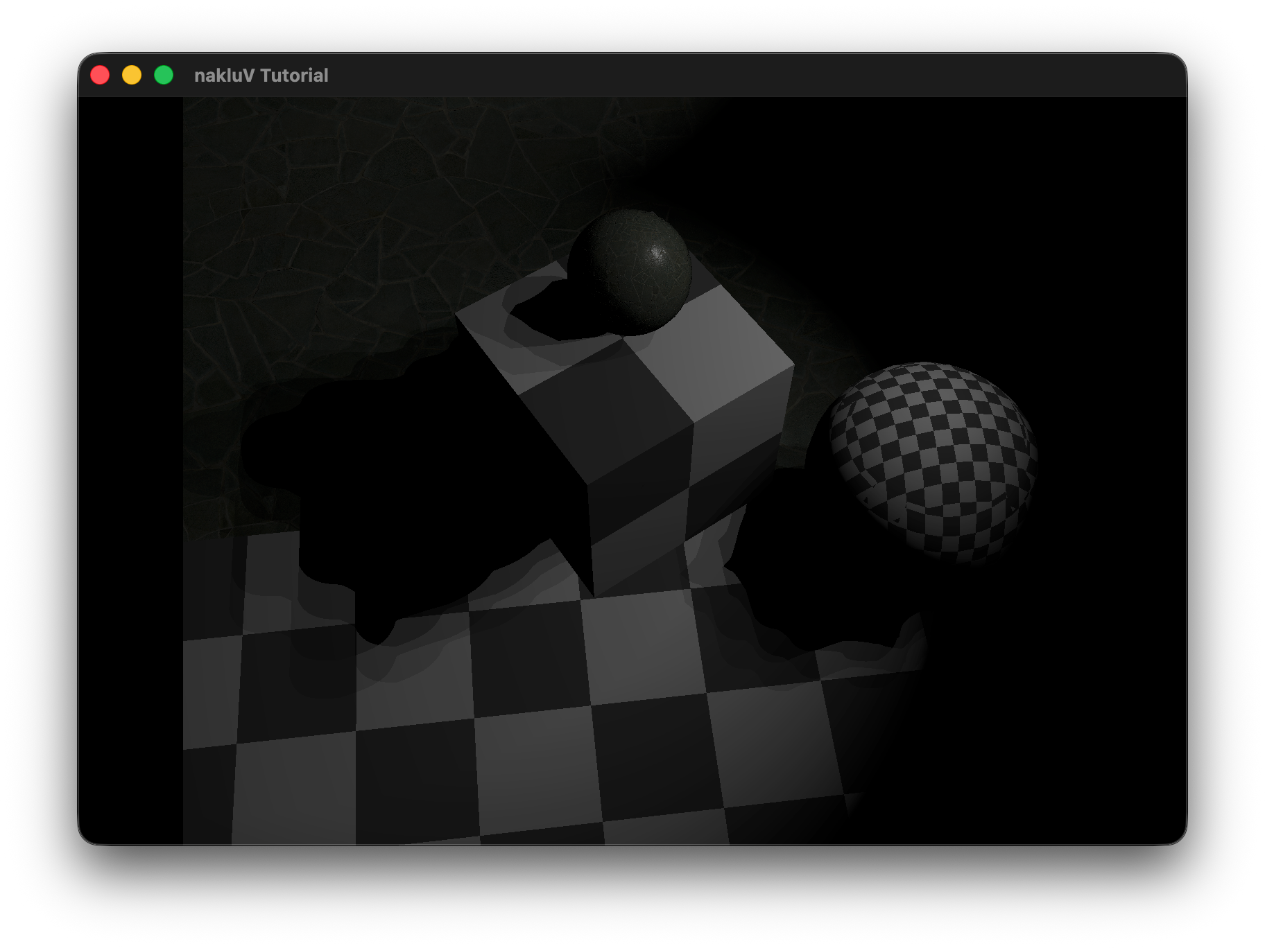
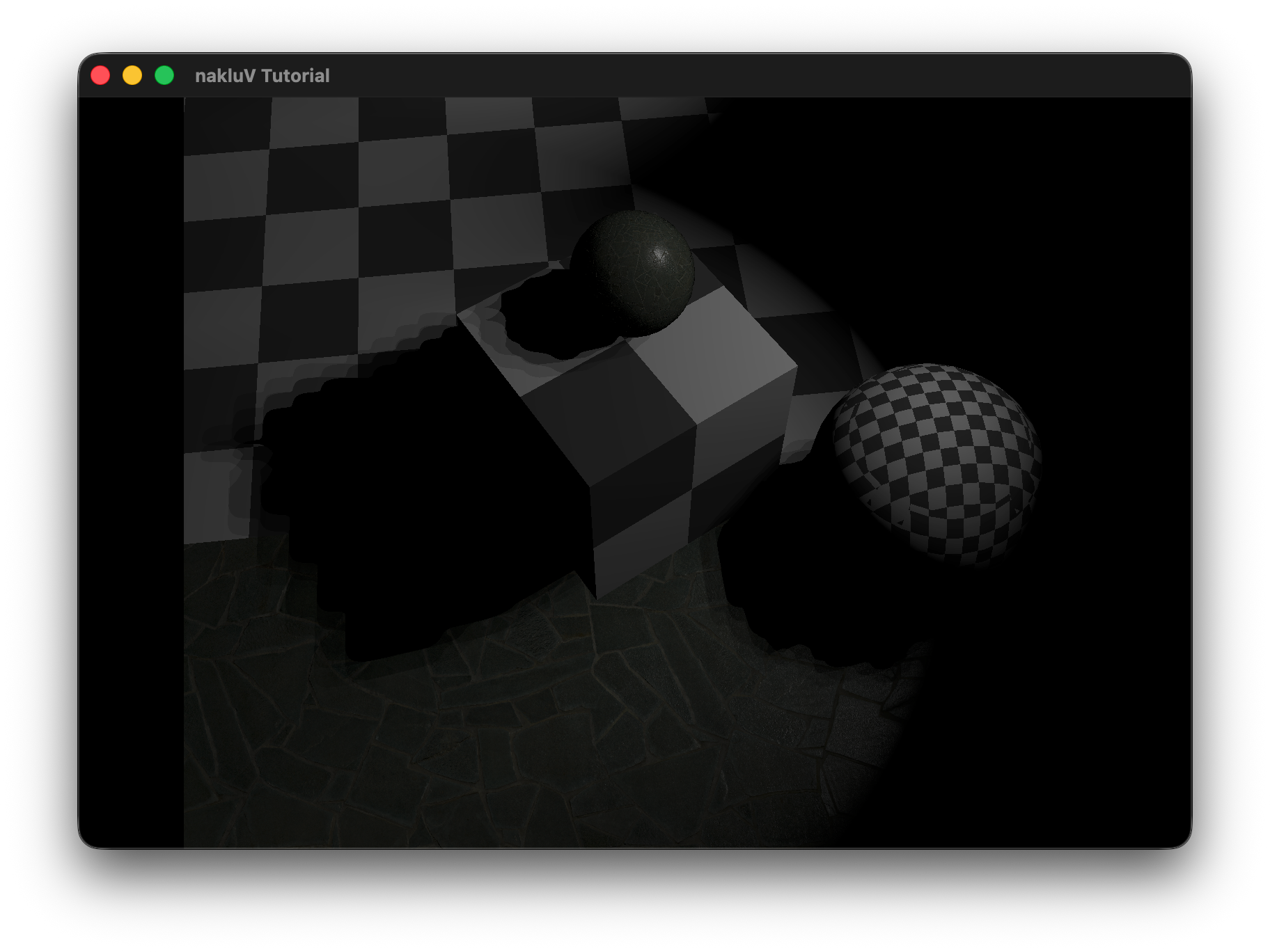
Build a scene in which your light sorting technique provides a performance improvement over rendering all meshes with all lights. Include a screen shot (and the scene itself).
Include data demonstrating the performance improvement in rendering this scene. E.g., a graph of the frame times for an animated fly-through of the scene with and without your sorting code enabled.
Cover, at least: your implementation of PCSS (sampling pattern, counts)
Include images showing the same shadows rendered with and without PCSS, showing the spreading behavior as the shadow stretches further from the light.
Cover, at least: your choice of shadow map cascade levels and layout; how your cascade is packed into a texture; how [if at all] your cascade avoids "boiling" as the camera moves
Include images showing a scene rendered with a shadow-casting distant directional light. Include images with a modified shader color-coding pixels by what cascade level they are sampling. Include images from a debug camera, showing how the shadow map cascade fits the camera frustum.
Cover, at least: how you chose to set up cameras for cube map rendering
Include images or video showing a scene rendered with a shadow-casting sphere light. Show that there are no artifacts at the edges or corners of the shadow map cube.
If you have received instructor permission to pursue another extra credit activity, include information about that activity here.
Include images or video showing a scene rendered with a shadow-casting sphere light. Show that there are no artifacts at the edges or corners of the shadow map cube.
This is the end of the structured report. Feel free to add feedback about A1 to this section.